A tiny proof for a tiny LLM

Jan 25, 2026

In this post, I’ll show you a tiny proof I used to convince myself I was using an API correctly.

While working through Tiny LLM - LLM Serving in a Week, I ran into the following question:

If a sampling API accepts logits, is it OK to pass in log-probabilities instead?

For my use case, the answer was yes! The proof in this post shows that:

Greedy decoding gives the same result from both logits and log-probabilities
MLX’s categorical sampling behaves identically in both cases.

More formally, given:

LogitsIf you’re new and are unsure about what logits are, scroll down and I’ll walk you through it. vector: $\vec{z}=\{z_1, \ldots, z_n\}$
Probability distribution: $\vec{p}=\text{softmax}(\vec{z})$ with $p_i = \frac{e^{z_i}}{\sum_{j}e^{z_j}}$
Logprobs $\vec{\ell}=\log(\vec{p})$

We’ll prove the two statements below:

Greedy decoding using either logits $\vec{z}$ or logprobs $\vec{\ell}$ as input will produce the same result. That is, $\underset{i}{\arg\max}{\space\vec{z}} = \underset{i}{\arg\max}{\space\vec{\ell}}$
The function mlx.core.random.categorical (Apple’s documentation) takes logits $\vec{z}$ as input, then:
1. Normalizes these logits into probabilities (via softmax), then
2. Samples from these probabilities.
Suppose you only had access to $\vec{\ell}$ and not $\vec{z}$. Show that applying mlx.core.random.categorical to $\vec{\ell}$ is equivalent.

Proof

If you’ve seen the derivation of a numerically stable softmax, this proof will look familiar. We’ll isolate a constant component and reason about what’s left.

For (1), given logprobs $\vec{\ell}=\log(\vec{p})$, we have that:

\[\ell_i = \log{p_i} = \log{\frac{e^{z_i}}{\sum_{j=1}^ne^{z_j}}} = z_i-\log{\sum_{j=1}^ne^{z_j}}\]

The second term, $\log{\sum_{j=1}^ne^{z_j}}$, is constant for all values of $i$, so we can set $M=\log{\sum_{j=1}^ne^{z_j}}$, giving us $\ell_i = z_i -M$.

Then:

\[\begin{aligned} \underset{i}{\arg\max}{\space\vec{\ell}} &= \underset{i}{\arg\max}\{\ell_1,\ldots,\ell_n\}\\ & = \underset{i}{\arg\max}\{z_1-M,\ldots,z_n - M\} && \small\text{(from above 👆)}\\ & = \underset{i}{\arg\max}\{z_1,\ldots,z_n\} && \substack{\text{(Adding }M\text{ doesn't change} \\ \text{where the max is)}}\\ & = \underset{i}{\arg\max}{\space\vec{z}} && \blacksquare \end{aligned}\]

To prove (2), note that when applying mlx.core.random.categorical to logits $\vec{z}$, it means we’re sampling from the probability distribution given by $\vec{p}=\text{softmax}(\vec{z})$.

Suppose we instead use $\vec{\ell}$ as input to mlx.core.random.categorical. This is equivalent to using $\vec{z}$ if and only if their probability distributions are the same, $\text{softmax}(\vec{z})=\text{softmax}(\vec{\ell})$.

Let $\vec{p}\prime=\text{softmax}(\vec{\ell})$. Then:

\[\begin{aligned} p\prime_i & = \frac{e^{\ell_i}}{\sum_{j=1}^ne^{\ell_j}} && \small\text{(definition of softmax)}\\ &= \frac{e^{z_i - M}}{\sum_{j=1}^ne^{z_j - M}} && \small\text{(above, we had $\ell_i = z_i -M$)}\\ &= \frac{e^M \cdot e^{z_i - M}}{e^M \cdot\sum_{j=1}^ne^{z_j - M}} && \small\text{(multiply top and bottom by $e^M$)}\\ &= \frac{e^{z_i}}{\sum_{j=1}^ne^{z_j}} && \small\text{(simplify)}\\ &= p_i && \small\text{(definition of $p_i$)} \end{aligned}\]

This holds for all values of $i\in\{1,\ldots,n\}$, which gives us $\text{softmax}(\vec{z})=\text{softmax}(\vec{\ell})$. Thus, when you use mlx.core.random.categorical here, it doesn’t matter whether you use logits or logprobs. $\blacksquare$

If you came here just to read a proof, you can skip everything below.

How did I get here?

Last summer, while stuck in prompt engineering purgatory at work, I got curious about how Large Language Models really worked on the inside.

I found Tiny LLM - LLM Serving in a Week, which features a “week long” (spoiler: it took me longer than a week) set of programming exercisesI later learned about Stanford’s CS336 “Language Modeling from Scratch”, which is packed with similarly good stuff and more. I look forward to going through that as well some time. where you implement Qwen2 from scratch using Apple’s mlx library.

The last section of Week 1 involves a small implementation of different sampling methods for decoding. For temperature sampling, the suggestion was to use mlx.core.random.categorical and pass in logprobs. I was confused because the documentation for this function says it accepts logits, so I spent a few minutes proving to myself that I could use either.

Are you out of the loop on LLMs?

I definitely was, and if you’re all the way down here reading this, you might be too. To put logits in context, it helps to zoom out and see where they come from in a modern LLM.

I found the diagram below to be helpful in visualizing how LLMs look on the inside. It comes from Sebastian Raschka’s blog post “The Big LLM Architecture Comparison”.

LLM Architecture Comparison

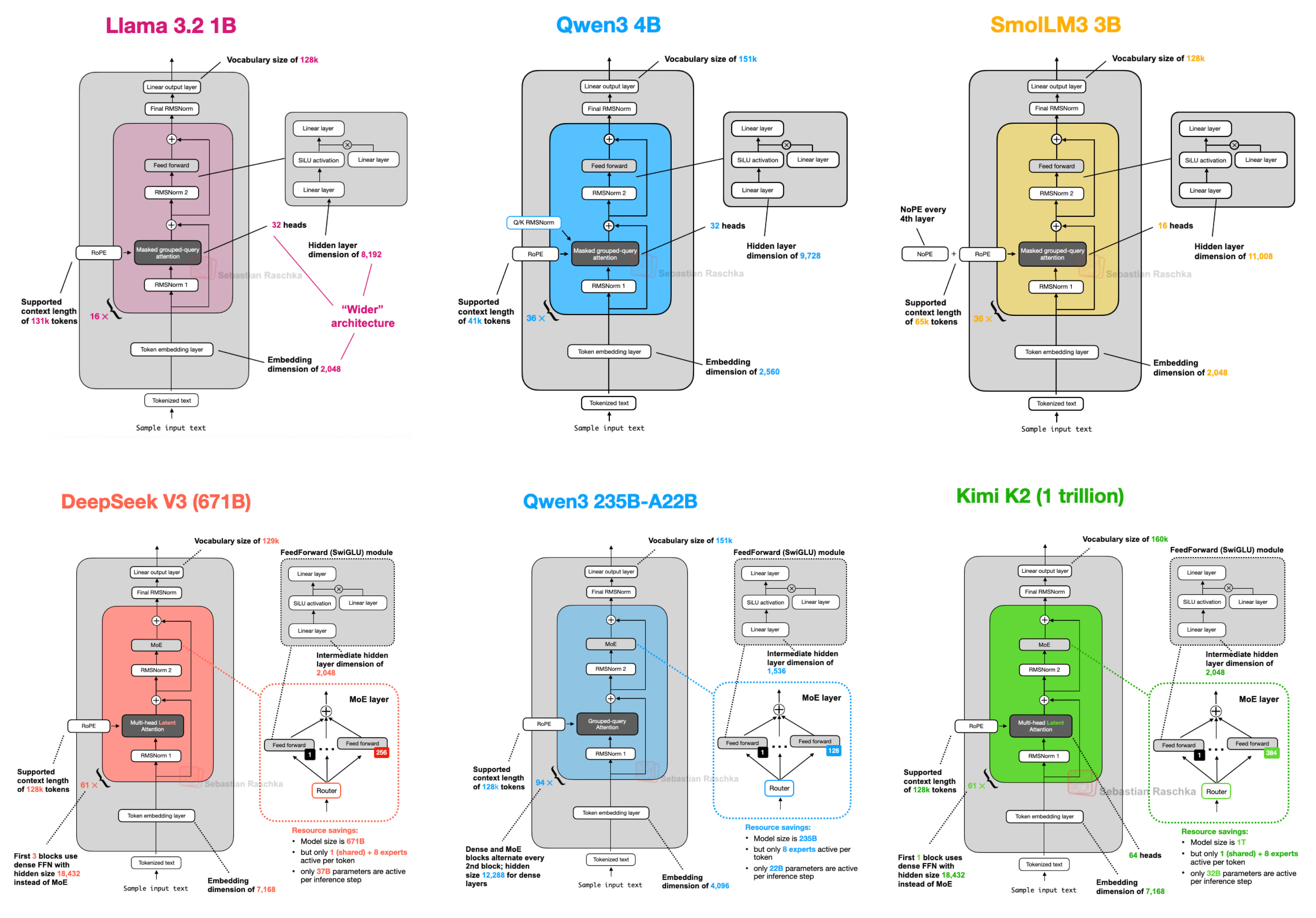
If you came here for an explanation of where logits come from, I’m going to make some generalizations about LLMs. LLMs take as input a sequence of tokens (which represents some text), and predict the next token that’s likely to follow. To accomplish this, most of the open source models follow a similar pattern:

From input tokens, get their embeddings
Go through several rounds of the following
1. Some type of attention mechanism
2. Normalization
3. Feedforward layer (Optionally: skip-connections, positional embeddings, and other optimizations)
More normalization
Linear layer

Qwen2 (from the Tiny LLM course), even though not mentioned in the blog above, follows the same pattern.

The output of step (4) includes logits $\vec{z}$, an $n$-dimensional vector ($n$ is the number of tokens in our vocabulary). Each component $z_i$ is an unnormalized ($z_i\in[-\infty,\infty]$) value; higher values correspond to tokens that are predicted to be more likely next in the sequence of text.

From here, it’s typical to compute $\vec{p}=\text{softmax}(\vec{z})$ with $p_i = \frac{e^{z_i}}{\sum_{j}e^{z_j}}$ (from the top), which gives us a probability distribution to sample from to produce the next token.